Moving Averages
As mentioned in the previous lesson, it is often advantageous to find average values of complicated data sets or functions in order to make reasonable predictions about what might happen in the future. However, as anyone in business will tell you, it is a VERY faulty assumption to think that trends and averages will stay the same over time. And furthermore, most of the time, such as if you’re watching the number of sales a company produces, you’d want your averages to move up over time!
Consider the function given by the graph below representing the number of new subscribers an online video streaming service acquires every day over the course of 36 months (3 years).
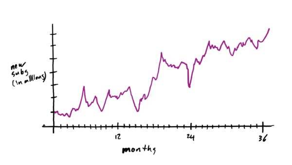
Firstly, notice that the trend of the data is generally upward over time, but with the occasional bad month. We might be interested in seeing what the average number of new subscribers is every three months throughout those three years. This would enable us to better see how the data is trending and perhaps enable us to make reasonable predictions about the average number of new subscribers over the next three months.
To do this, we could compute the average value of the function using the integral method described in the previous lesson for every 3-month time interval. See the table below for how this might work out. Note that the numbers are estimates from the graph, not actual computations. Just want to illustrate a point for now.
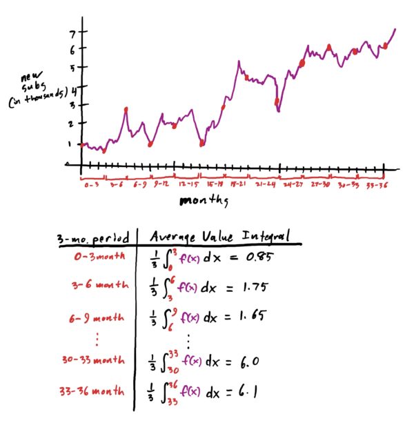
Notice that the only thing that changes in any of our calculations is where the integral starts and stops. Notice also that the upper limit for the integral was always 3 greater than the lower limit (because we’re finding the average value of the function every three months, starting on every third month). So, if you think about it for a moment, you might realize that the only thing that really changes here in all these calculations is the starting/lower limit of the integral. Thus, if we wanted to start at some arbitrary \(t\)-value, we could find the average value of the function \(f\) over the following \(3\) months by computing
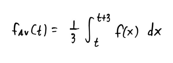
Since this starting point \(t\) can be any value between 0 and 36 months, we get that the above integral is actually a function in \(t\) that calculates the average value of \(f\) from whatever starting point \(x\) to 3 months later. Furthermore, because this is a function, it can be graphed by point-plotting. This moving average function is graphed below, with bigger points drawn at the three-month-marks to reflect what we had in the table.

In essence, this function and its graph “smooth out the data,” giving us a more clear picture as to how the data is trending on a three-month basis. In general, the following definition gives us a formula for computing the moving average of any function over any time-frame.
When we have a function given to us by a rule rather than a data set, we actually can get a function that looks “nicer” than the integral you see above.
Since \(x\) represents “days elapsed,” building a one-week moving average makes our \(p\) in the moving average formula equal to \(7\) (because 7 days in a week). Thus, the moving average is computed as follows.
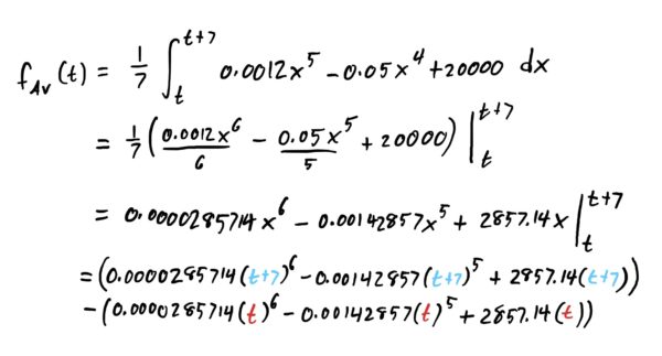
Thus, with a little simplifying of the above, we see that our 7-day moving average is the following function:
$$f_{Av}(t)=0.0000285714[(t+7)^6-t^6]-0.00142857[(t+7)^5-t^5]+20000$$
While certainly not the prettiest thing in the world, it gets the job done! Now, we can use it to calculate the average value of our function \(f\) over any 7-day period, starting at day \(t\) simply by plugging in different values for \(t\). Since we want the 7-day average starting at day \(235\), simply let \(t=235\) in the above function to get your answer!
$$f_{Av}(235)=764862000$$
Done!
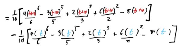
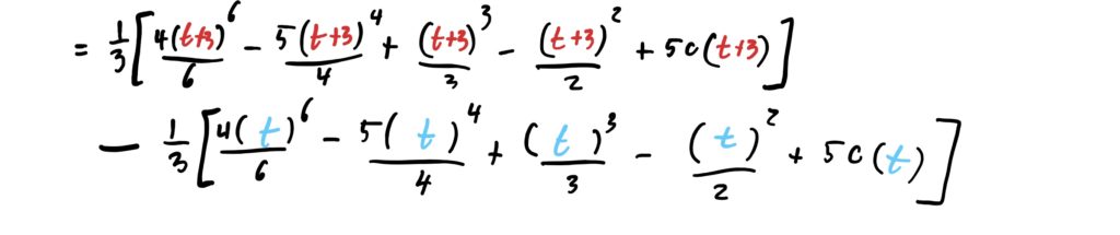
Use the formula for moving averages and let \(p=3\). Carry out the entire integral as usual.
The \(p\)-unit moving average of a function is given by:
$$f_{Av}(t)=\frac{1}{p}\int_{t}^{t+p}f(x)\ dx$$
Use the formula for moving averages and let \(p=10\). Carry out the entire integral as usual.
The \(p\)-unit moving average of a function is given by:
$$f_{Av}(t)=\frac{1}{p}\int_{t}^{t+p}f(x)\ dx$$