Graphing (Simple) Logarithmic Functions
Graphs of Logarithmic Functions
Because we can define functions using logarithms, and such functions are defined for all input \(x\)-values greater than \(0\), it only makes sense that we can graph logarithmic functions.
The graphs of logarithmic functions and their shape (along with locations of its “control points”) are entirely dictated by the base of the logarithmic function. Below we illustrate the key differences along with some of the key features of these two sorts of graphs. This will augment our library of functions considerably!

\(f(x)=\log_a(x)\) where \(a>1\)
Key Features:
- Has a concave-downward, rapidly-and-then-slowly increasing general shape you see at left (when the base \(a>1\)).
- The graph will NEVER cross the \(y\)-axis, but it will get as close as you like to it from the right as \(x\)-value inputs get closer and closer to zero. This gives a vertical asymptote at \(x=0\).
- As \(x\)-value inputs get bigger, the \(y\)-values slowly get bigger. It takes very large inputs to produce relatively small outputs.
- As the \(x\)-value inputs get smaller, the \(y\)-values decrease rapidly.
Control/Reference Points
The graph of \(f(x)=\log_a(x)\) passes through \((\frac{1}{a},-1)\), \((1,0)\), and \((a,1)\).
The graph at left shows the function \(f(x)=\log_2(x)\) which has control points \((\frac{1}{2},-1), (1,0),\) and \((2,1)\).
\(f(x)=\log_a(x)\) where \(a<1\)
Key Features:
- Has a concave-upward, rapidly-and-then-slowly decreasing general shape you see at right (when the base \(a<1\)).
- The graph will NEVER cross the \(y\)-axis, but it will get as close as you like to it from the right as \(x\)-value inputs get closer and closer to zero. This gives a vertical asymptote at \(x=0\).
- As \(x\)-value inputs get bigger, the \(y\)-values slowly get more and more negative. It takes very large inputs to produce relatively small negative outputs.
- As the \(x\)-value inputs get smaller (i.e. closer to zero), the \(y\)-values increase rapidly.
Control/Reference Points
The graph of \(f(x)=\log_a(x)\) passes through \((\frac{1}{a},-1)\), \((1,0)\), and \((a,1)\).
The graph at left shows the function \(f(x)=\log_{\frac{1}{2}}(x)\) which has control points \((\frac{1}{\frac{1}{2}},-1)=(2,-1), (1,0),\) and \((\frac{1}{2},1)\).

To reiterate the above, the graph and thus the control points used to graph a logarithm are determined by the base \(a\). It’s helpful to try listing the control points of various functions of the form \(f(x)=\log_a(x)\) for different \(a\)-values so that you see a pattern in how they are computed. Note that regardless of whether \(a>1\) or \(a<1\), the control points are calculated the same way. See below.
| Logarithmic Function | \(a\)-value (base) | Control Points: \((\frac{1}{a},-1)\), \((1,0)\), \((a,1)\) |
| \(f(x)=\log_\frac{1}{3}(x)\) | \(a=\frac{1}{3}\) | \((\frac{1}{a},-1)=(3,-1)\), \((1,0)\), \((a,1)=(\frac{1}{3},1)\) |
| \(f(x)=\log_{\frac{1}{2}}(x)\) | \(a=\frac{1}{2}\) | \((\frac{1}{a},-1)=(2,-1)\), \((1,0)\), \((a,1)=(\frac{1}{2},1)\) |
| \(f(x)=\log_\frac{2}{3}(x)\) | \(a=\frac{2}{3}\) | \((\frac{1}{a},-1)=(\frac{3}{2},-1)\) ,\((1,0)\), \((a,1)=(\frac{2}{3},1)\) |
| \(f(x)=2^x\) | \(a=2\) | \((\frac{1}{a},-1)=(\frac{1}{2},-1)\), \((1,0)\), \((a,1)=(2,1)\) |
| \(f(x)=\log_5(x)\) | \(a=5\) | \((\frac{1}{a},-1)=(\frac{1}{5},-1)\), \((1,0)\), \((a,1)=(5,1)\) |

First find the control points and plot those. The control points are \((\frac{1}{a},-1)=(\frac{1}{3},-1)\), \((1,0)\), \((a,1)=(3,1)\), since \(a=3\). Since the base is greater than \(1\), the \(y\)-values of the function increase as the input \(x\)-values increase. This gives the graph the shape you see below once you draw through the plotted control points. Note that the graph has a vertical asymptote at \(y=0\); i.e. it doesn’t cross the \(y\)-axis EVER!

First find the control points and plot those. The control points are \((\frac{1}{a},-1)=(3,-1)\), \((1,0)\), \((a,1)=(\frac{1}{3},1)\), since \(a=\frac{1}{3}\). Since the base is less than \(1\), the \(y\)-values of the function decrease as the input \(x\)-values increase. This gives the graph the shape you see below once you draw through the plotted control points. Note that the graph has a vertical asymptote at \(y=0\); i.e. it doesn’t cross the \(y\)-axis EVER!

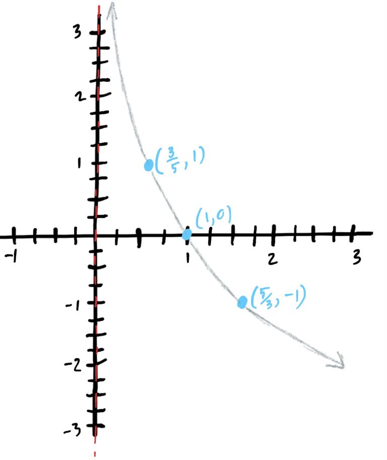
First find the control points and plot those. Feel free to use a calculator to calculate a decimal value for some of these fractions. The control points are \((\frac{1}{a},-1)=(\frac{5}{3},-1)\), \((1,0)\), \((a,1)=(\frac{3}{5},1)\), since \(a=\frac{3}{5}\). Since the base is less than \(1\), the \(y\)-values of the function decrease as the input \(x\)-values increase. This gives the graph the shape you see below once you draw through the plotted control points. Note that the graph has a vertical asymptote at \(y=0\); i.e. it doesn’t cross the \(y\)-axis EVER!

First find the control points and plot those. Note that \(\ln(x)=\log_e(x)\), where \(e=2.71828…\). The control points are \((\frac{1}{a},-1)=(\frac{1}{e},1)\approx (0.3678797,-1)\), \((1,0)\), \((a,1)=(e,1)\approx (2.71828,1)\), since \(a=e\). Since the base is greater than \(1\), the \(y\)-values of the function increase as the input \(x\)-values increase. This gives the graph the shape you see below once you draw through the plotted control points. Note that the graph has a vertical asymptote at \(y=0\); i.e. it doesn’t cross the \(y\)-axis EVER!