Graphing (Simple) Exponential Functions
Graphs of Exponential Functions
More often than not, it is easier to graph a function (or a class of functions) once you know something about the shape of the function and perhaps a few points on the graph itself. Similar to how we graph lines by essentially plotting two reference points and drawing a straight line through them, so too can we graph exponential functions. However for exponential functions we use three reference points, which we will refer to as “control points,” and a few other key facts about exponential functions (explained below).
The graphs of exponential functions and their shape (along with locations of its “control points”) are entirely dictated by the base of the exponential function. Below we illustrate the key differences along with some of the key features of these two sorts of graphs. This will augment our library of functions considerably!
\(f(x)=a^x\) where \(a>1\)
Key Features:
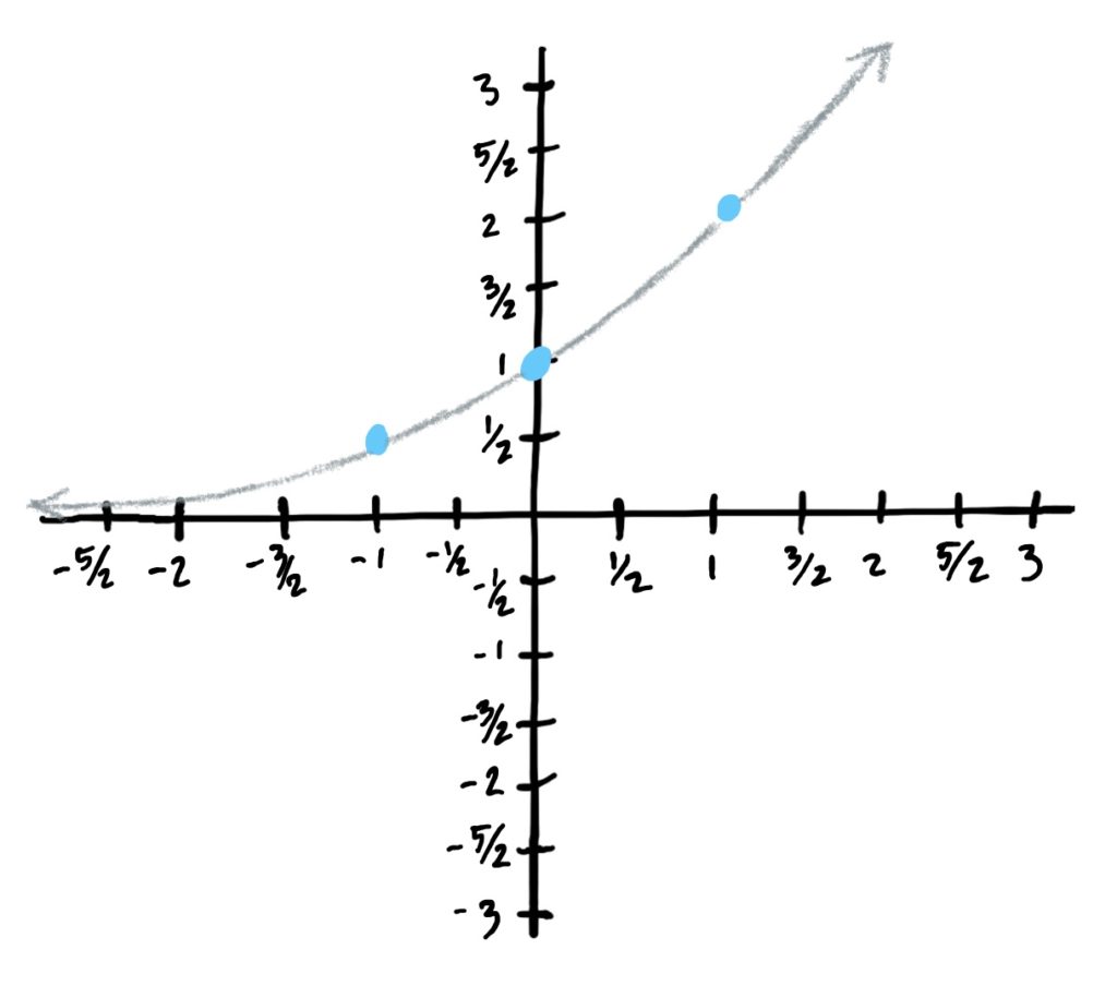
- Has a concave-upward, increasing general shape you see at left regardless of the base.
- The graph will NEVER cross the \(x\)-axis, but it will get as close as you like to it from above as \(x\)-value inputs get more and more negative. This gives a horizontal asymptote at \(y=0\).
- As \(x\)-value inputs get bigger, the \(y\)-values explode into the sky (i.e. increase quickly).
Control/Reference Points
The graph of \(f(x)=a^x\) passes through \((-1,\frac{1}{a})\), \((0,1)\), and \((1,a)\).
The graph at left shows the function \(f(x)=2^x\) which has control points \((-1,\frac{1}{2}), (0,1),\) and \((1,2)\).
\(f(x)=a^x\) where \(a<1\)
Key Features:
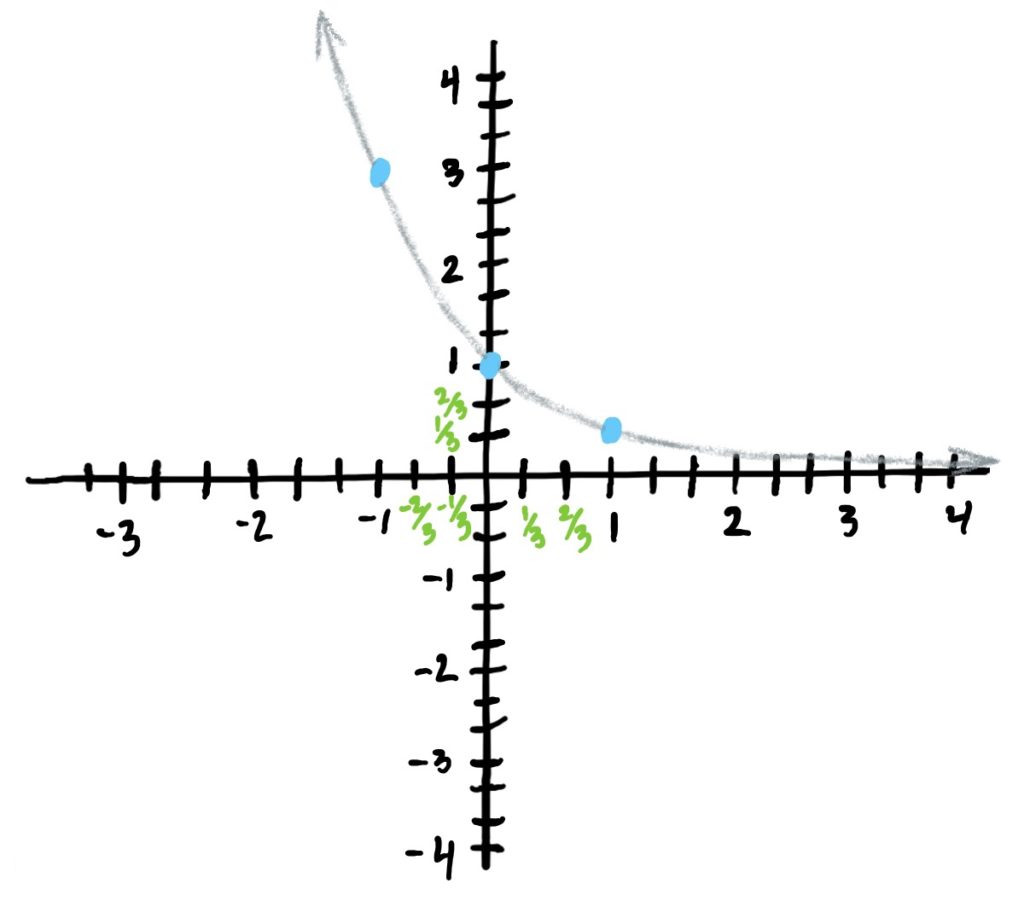
- Has a concave-upward decreasing general shape.
- The graph will NEVER cross the \(x\)-axis, but it will get as close as you like to it from above as \(x\) gets more and more positive. This gives a horizontal asymptote at \(y=0\).
- As \(x\)-value inputs get bigger, the \(y\)-values decrease more slowly, tending toward \(y=0\).
Control/Reference Points
The graph of \(f(x)=a^x\) passes through \((-1,a)\), \((0,1)\), and \((1,\frac{1}{a})\).
The graph at right is the graph of the function \(f(x)=\left(\frac{1}{3}\right)^x\), which has control points \((-1,3), (0,1), (1,\frac{1}{3})\)
To reiterate the above, the graph and thus the control points used to graph an exponential are largely determined by the base \(a\). It’s helpful to try listing the control points of functions of the form \(f(x)=a^x\) for different \(a\)-values so that you see a pattern in how they are computed. Note that regardless of whether \(a>1\) or \(a<1\), the control points are calculated the same way. See below.
| Exponential Function | \(a\)-value (base) | Control Points: \((-1,\frac{1}{a})\), \((0,1)\), \((1,a)\) |
| \(f(x)=\left(\frac{1}{3}\right)^x\) | \(a=\frac{1}{3}\) | \((-1,3)\), \((0,1)\), \((1,\frac{1}{3})\) |
| \(f(x)=\left(\frac{1}{2}\right)^x\) | \(a=\frac{1}{2}\) | \((-1,2)\), \((0,1)\), \((1,\frac{1}{2})\) |
| \(f(x)=\left(\frac{2}{3}\right)^x\) | \(a=\frac{2}{3}\) | \((-1,\frac{3}{2})\) (because \(\frac{1}{\frac{2}{3}}=\frac{3}{2}\)), \((0,1)\), \((1,\frac{2}{3})\) |
| \(f(x)=2^x\) | \(a=2\) | \((-1,\frac{1}{2})\), \((0,1)\), \((1,2)\) |
| \(f(x)=5^x\) | \(a=5\) | \((-1,\frac{1}{5})\), \((0,1)\), \((1,5)\) |

First find the control points and plot those. The control points are \((-1,\frac{1}{a})=(-1,\frac{1}{3})\), \((0,1)\), \((1,a)=(1,3)\), since \(a=3\). Since the base is greater than \(1\), the \(y\)-values of the function increase as the input \(x\)-values increase. This gives the graph the shape you see below once you draw through the plotted control points. Note that the graph has a horizontal asymptote at \(y=0\); i.e. it doesn’t cross the \(x\)-axis EVER!


First find the control points and plot those. The control points are \((-1,\frac{1}{a})=(-1,5)\), \((0,1)\), \((1,a)=(1,\frac{1}{5})\) since \(a=\frac{1}{5}\). Since the base is less than \(1\), the \(y\)-values of the function decrease as the input \(x\)-values increase. This gives the graph the shape you see below once you draw through the plotted control points. Note that the graph has a horizontal asymptote at \(y=0\); i.e. it doesn’t cross the \(x\)-axis EVER!


First find the control points and plot those. The control points are \((-1,\frac{1}{a})=(-1,\frac{5}{3})\) (because \(\frac{1}{\frac{3}{5}}=\frac{5}{3}\) by keep-change-flip method), \((0,1)\), \((1,a)=(1,\frac{3}{5})\), since \(a=\frac{3}{5}\). Since the base is less than \(1\), the \(y\)-values of the function decrease as the input \(x\)-values increase. This gives the graph the shape you see below once you draw through the plotted control points. Note that the graph has a horizontal asymptote at \(y=0\); i.e. it doesn’t cross the \(x\)-axis EVER!