Graphing Lines

All linear functions and all linear equations can be written in the form \(y=mx+b\), called slope intercept form, where \(m\) is the slope or rate of change of the line, and \(b\) is the \(y\)-intercept of the line.

The rate of change \(m\) tells you how much the \(y\)-values of the function change given a certain change in \(x\).

For example, if given the equation for the line \(y=\frac{2}{3}x+1\), the slope is \(m=\frac{2}{3}\) which means “for every 3 I move to the right (i.e. change in \(x\)) from a chosen point on the line, I should move up 2 to land on another point on the line.”

To graph linear functions in slope intercept form \(f(x)=mx+b\), either use the method described in the video (easier), or do the following:

1. First, plot the \(y\)-intercept \(b\) on the \(y\)-axis, noting that the line will cross through this point.
   • Aside: The reason the line crosses through this point is because \(f(0)=m(0)+b=b\); that is, when you plug in \(x=0\), and graph the corresponding \(y\)-value, you end up plotting \(y=b\) on the \(y\)-axis.
2. Turn the slope into a fraction (if not already a fraction), by dividing the whole number (or decimal) by 1. (e.g. if the slope is \(m=3\) in the line equation, write instead \(m=\frac{3}{1}\).
3. From the \(y\)-intercept you plotted, move to the right from that point according to the denominator of your slope, as found in the last step. Then, move up according to the value of the numerator of the slope found in the last step; plot a point there.
4. Draw a line through both the \(y\)-intercept and the point just plotted so that the line extends infinitely in both directions.

Special Considerations:

If the function is constant (e.g. \(f(x)=5\)), then the graph is a flat line through the \(y\)-axis at \(y=5\).

This is because constant functions can be written as linear functions of the form \(f(x)=0x+b\), so no matter what the \(x\)-value is that is being plugged in, the output is always the same value, namely \(b\).

Such lines have zero slope.

Vertical lines can be written in the form \(x=c\) where \(c\) is a real number. Note that such lines do not represent a function of \(x\), but they DO represent a constant (and therefore linear function) in \(y\).

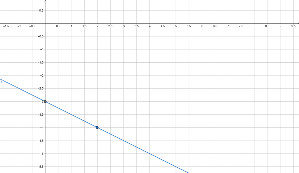
The examples below are practice for plotting lines from the slope-intercept form of a given function \(f(x)=mx+b\).