First Derivative Test for Finding Local Mins and Maxes

Critical Points

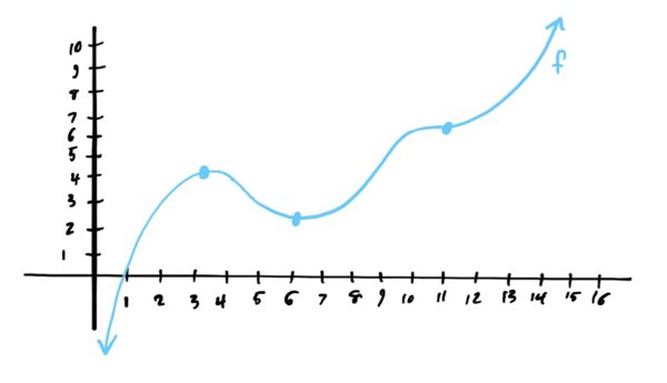
Take a look at the graph below and locate the local/relative mins and maxes. If we draw a line that is tangent to the graph at each of these points, what do you notice about their slopes?

Looking at the slope of these tangent lines, we notice that the slopes are ZERO! This makes sense, because as a function goes from increasing to decreasing (when reading the graph from left to right) there needs to be that “turning point.” Since most of the graphs and functions we deal with are smooth (i.e. no cusps or hard corners), we can identify where we may have a local min or max simply by considering where we have tangent lines with zero slope (which is precisely when the function itself has “zero slope). This is useful when we don’t have a graph handy, or when using a graph to locate extrema would yield inaccurate results.

Remember that the derivative \(f’\) can be thought of as a “slope formula” or a rule that tells you the slope of \(f\) at any given \(x\)-value. Since local extrema of smooth functions are where the function has zero slope (i.e. where it is neither increasing nor decreasing) we now have a modestly easy way of finding where said extrema could reside.

Quick Example: Find the critical points of the function \(f(x)=-3x^3+2x+1\) on the interval \((-\infty,\infty)\)

When we are asked to find the critical points of a function, we are looking for all \(x\)-values where the derivative is zero. So, we first compute the derivative of the given function and set it equal to zero, and then solve for \(x\) using whatever algebraic techniques we have at our disposal. See below.

$$f'(x)=-9x^2+2$$

Setting this equal to zero:

$$-9x^2+2=0$$

Now, solve for \(x\):

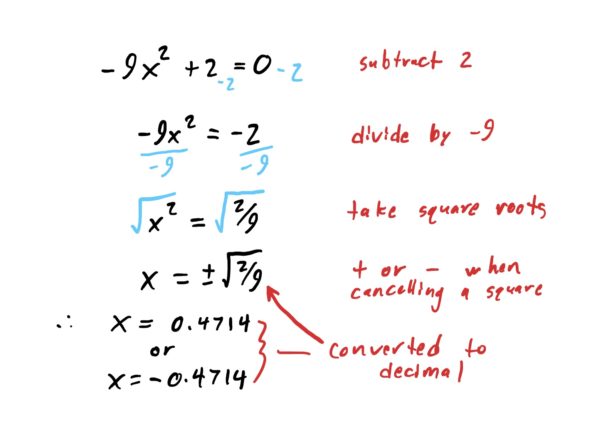
So, we therefore have two critical points: \(x=-0.4714\) and \(x=0.4714\). At these critical points we may have a min, max or “neither.” The next section is all about determining whether a critical point is one of these three options.

Classifying Critical Points as Min, Max, or Neither

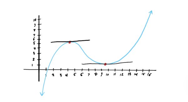
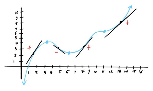
Take a look at the graph below, and locate the critical points.

Note that we have critical points \(x=3,6,\) and \(x=11\). \(x=3\) is a local max, \(x=6\) is a local min, and \(x=11\) is neither (but it is still a critical point because the slope is zero at \(x=11\).

Now, in effort to develop some intuition for how we can determine whether a critical point is a min, max, or neither, lets look at the slopes before and after these critical points. The “+” on the graph below indicates that the slope of the graph is positive (i.e. the graph is increasing), whereas a “-” indicates that the slope of the graph is negative (the graph is decreasing).

Notice that before the local max \(x=3\), the slope is positive. After \(x=3\) (but before the next critical point), the slope of the graph is negative. So the graph is going uphill until \(x=3\), then starts heading downhill after \(x=3\). This characterizes \(x=3\) as a local max: “up, then back down.”

Notice that just before \(x=6\) the slope of the graph is negative, and afterward it is positive. This indicates that we have a local min at \(x=6\): “down, then back up.”

Lastly, at \(x=11\), the slope of the graph is positive leading up to \(x=11\), flattens out at exactly \(x=11\), and then continues increasing afterward. This indicates that \(x=11\) is neither a local min nor a max because we get neither a hill nor a valley at \(x=11\).

All of this is summarized in the following theorem.

We usually use a number line to help with classifying critical points according to the above theorem. See the next example.

Quick Example: Find the critical points of the function \(f(x)=-3x^3+2x+1\) on the interval \((-\infty,\infty)\) and classify them as local mins, maxes or neither.

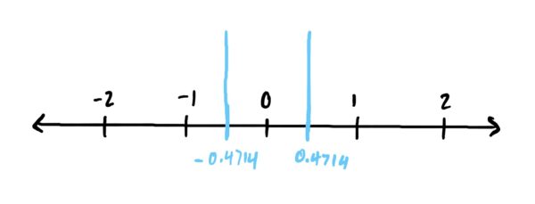
First things first: we need to find the critical points before we can classify them. Thankfully, we already did this in a prior example. We found that the critical points are: \(x=0.4714\) and \(x=-0.4714\). Now we need to classify them. We do this using a number line.

Start by plotting the critical points on the number line. I like to do this with long vertical lines.

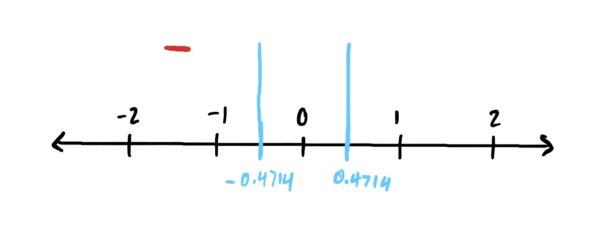
Lets first classify \(x=-0.4714\). Using the first derivative test, we need to determine whether the derivative is positive or negative to the left and right of \(x=-0.4714\). Choose an \(x\)-value to the left of \(x=-0.4714\) and plug it into \(f’\) and see if you get a positive number or a negative number. If positive, draw a little “+” to the left of \(x=-0.4714\), if negative, draw a “-” to the left of \(x=-0.4714\). I chose \(x=-1\) which is less than \(x=-0.4714\) (i.e. to the left of \(x=-0.4714\)).

\(f'(-1)=-9(-1)^2+2=-7\) which is negative. Draw a minus sign to the left of \(x=-0.4714\)

Now, do the same thing on the right of \(x=-0.4714\), choosing a number greater than \(x=-0.4714\) (but also less than \(x=0.4714\)) so we can determine whether the slope is positive or negative between the critical points. I chose \(x=0\). Thus,

\(f'(0)=-9(0)^2+2=2\) which is positive. Thus, we draw a “+” between our critical points to show that \(f\) is increasing there.

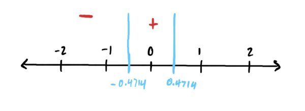
At this point, since \(f\) is decreasing (negative slope) before \(x=-0.4714\) and increasing after \(x=-0.4714\) (positive slope) this means we have a local min at \(x=-0.4714\).

Now, we repeat the process for the critical point \(x=0.4714\). We already know by our number line that \(f\) is increasing to the left of \(x=0.4714\). So we choose a number to the right of \(x=0.4714\) and plug it into \(f’\) to determine what is happening to the right of \(x=0.4714\). I chose \(x=1\).

\(f'(1)=-9(1)^2+2=-7\) which is negative, which means that the slope of \(f\) is negative after \(x=0.4714\). We indicate this with a “-” on the number line.

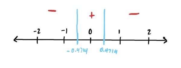
Thus, looking at our number line, we have that \(x=0.4714\) is a local max because \(f\) is increasing before \(x=0.4714\) and decreasing afterward.

Therefore, we have: local min at \(x=-0.4714\), and local max at \(x=0.4714\). Done.

If you find it more helpful to have all your “+” and “-” on your number line before you start classifying things as maxes or mins you certainly can. Its just a matter of preference.

Classifying Endpoints of an Interval

Some problems may ask you to also classify the endpoints of an interval as a local min or max in addition to critical points. This is easy, as the number line method we used before indicates whether the function is increasing or decreasing around different points, including interval endpoints.

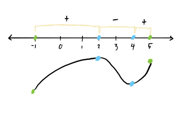
For example, suppose we are working on a problem that asks “Find and classify all critical points AND endpoints of the function \(f\) on the interval \([-1,5]\).” Throughout the problem, suppose we found our critical points at \(x=2\) and \(x=4\) and drew our number line as follows, plotting critical points AND endpoints:

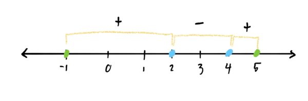
Note that because the function is increasing after \(x=-1\), that makes the endpoint \(x=-1\) a local min. Similarly, because we are increasing up to \(x=5\), that would make \(x=5\) a local max. The function would have the sort of shape you see below, based on this number line.