$Project Greater Ed Logo$

Basic Definitions and Concepts

Discrete Mathematics Graph Theory Basics Basic Definitions and Concepts

Representing a Graph, well, Graphically

Graph (and other related definitions)

A Graph $G=(V(G),E(G))$ is a pair of two finite sets: a set $V(G)$ of vertices and a set $E(G)$ of edges, where each element (edge) of $E(G)$ is associated with one or two elements of $V(G)$, which are called endpoints of the edge.

For the sake of procedures and algorithms, and for the sake of mathematical precision we use the above definition. But more often than not we represent graphs, well, graphically, plotting our vertices from the vertex set $V(G)$ wherever we please on a piece of paper and connecting the vertices with the edges listed in the edge set $E(G)$.

Solution:

Note that there are many ways you could organize your vertices. This is something that will be discussed in more detail in future topics.

In the example above, we saw that between the vertices $a$ and $b$, there were two different edges. A pair of edges that have the same endpoints are called parallel edges. Also, in the example above, we had the edge $e_6$ which had the endpoints $c$ and $c$ (i.e. the edge “started where it ended”). An edge with only one distinct endpoint is called a loop.

Two vertices that are endpoints of the same edge are said to be adjacent (such as with vertices $v_1$ and $v_4$ above). A vertex that is the endpoint of a loop is said to be self-adjacent. Also, an edge is said to be incident on each of its endpoints, and any pair of edges that are incident on the same vertex are adjacent edges (for example, $e_1$ and $e_2$ are adjacent edges in the graph above).

It is possible to have a graph that has a “floating vertex,” called an isolated point. It is also possible to have a graph with no vertices and no edges. Such a graph is called an/the empty graph. See below.

Note

Graphs need not be “completely connected” in some way. A single graph could consist of several “smaller” graphs that not at all connected in any way. See graph $G_1$ in the above picture This idea will be made more precise in future lessons.

Converting a Graph to its Set Notation

Just like how we can take a list of vertices and edges that define a graph and draw a graphical representation of it, so too can we take a graphical representation of a graph and write it as a list of vertices and edges. For a given graph $G$, this is done by adding all vertices of the diagram to the vertex set $V(G)$ of $G$, and adding all edges in the diagram to the edge set $E(G)$ of $G$, and listing the endpoints that each edge is associated with.

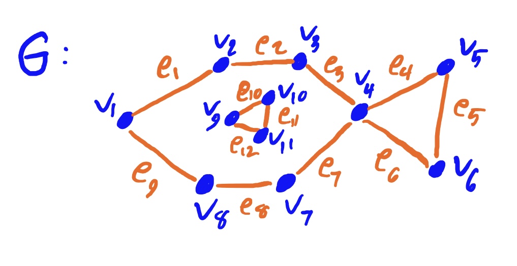
Problem: Let $G$ be the graph depicted below. Write all elements of $V(G)$ and $E(G)$, and list the endpoints associated with each edge.

Answer:

$V(G)=\{v_1,v_2,v_3,v_4,v_5,v_6\}$

$E(G)=\{e_1,e_2,e_3,e_4,e_5\}$ where each edge corresponds to the sets with the following end points.

$$\begin{align}e_1&:\{v_2,v_3\}\\e_2&:\{v_1,v_3\}\\e_3&:\{v_4,v_4\}\\e_4&:\{v_2,v_4\}\\e_5&:\{v_2,v_6\}\end{align}$$

Degrees and the Handshake Theorem

There are many useful theorems that come as a result of considering “how connected” a graph is, by counting vertices, edges, and the number of edges incident to specific vertices.

Degree and Total Degree

Let $G$ be a graph and let $v\in V(G)$. The degree of $v$, denoted deg$(v)$, is the number of edges incident to $v$, (where loops are counted twice). The total degree of $G$, which we will denote as Tot$(G)$, is the sum of degrees of all vertices in the graph.

Note that isolated points have degree zero.

Think of degree of a vertex $v$ as the total number of lines leaving $v$, regardless of where the lines go (even if they loop back around to the same point).

In the above graph, the degree of $v_1$ is $5$. The total degree of $G$ is $12$. Notice that the total degree, in this case, is twice the number of edges in the graph. It turns out that this is the case no matter what graph you are looking at! The following theorem makes this official.

Handshake Theorem

Let $G$ be a graph with vertices $v_1,v_2,v_3,…,v_n$. Then
$$\begin{align} \text{Tot}(G)&=\sum_{v\in V(G)}\text{deg}(v)\\&=\text{deg}(v_1)+\text{deg}(v_2)+…+\text{deg}(v_n)\\&=2\cdot |E(G)| \end{align}$$

Proof: Let $G$ be an arbitrary graph. Lets first suppose that $G$ is empty or consists of ONLY isolated vertices. Then there are no edges (by definition of empty graph or isolated vertices). Therefore the total degree of $G$ is zero, which equals $2$ times the number of edges (zero edges).

Now suppose that $G$ has $n$ vertices, and $m\geq 1$ edges, (where $n,m\in \mathbb{N}$). Let $e$ be an arbitrarily chosen edge in $E(G)$, with endpoints $v,w\in V(G)$. If $v\neq w$, then $e$ contributes $1$ to both the degree of $v$ and the degree of $w$ (and therefore adds $2$ to the total degree). If $v=w$, then $e$ is a loop, and therefore $e$ adds $2$ to the degree of $v$ and therefore adds $2$ to the total degree of the graph. Since an edge can only connect a vertex to itself or one vertex to exactly one other distinct vertex, no matter what, $e$ must contribute $2$ to the total degree of the graph. Since $e$ was arbitrarily chosen (i.e. there isn’t anything special about $e$ compared to any other edge), it follows that any/all edges in a graph must contribute $2$ to the total degree. Therefore, the total degree of $G$ is twice the number of edges in $E(G)$. This proves the original statement. QED

$V(G)=\{v_1,…,v_8\}$ and $E(G)=\{e_1,…,e_12\}$ where each edge is associated with the following endpoints: $e_1:\{v_1,v_2\}$, $e_2:\{v_2,v_3\}$, $e_3:\{v_3,v_4\}$, $e_4:\{v_4,v_5\}$, $e_5:\{v_5,v_6\}$, $e_6:\{v_6,v_4\}$, $e_7:\{v_4,v_7\}$, $e_8:\{v_7,v_8\}$, $e_9:\{v_8,v_1\}$, $e_{10}:\{v_9,v_{10}\}$, $e_{11}:\{v_{10},v_{11}\}$, $e_{12}:\{v_{11},v_9\}$

Note that your order of endpoints might differ from the ones listed above. Since this is a normal graph (undirected), the order endpoints are listed in each edge does not matter.

deg$(v_4)=4$

deg$(v_9)=2$

Total degree of $G$: $24$

Remember that the degree of a vertex is the number of edges that a vertex has coming out of it.

The total degree of a graph is the sum of the degrees of all its vertices.

Previous Lesson

Back to Lesson

Next Topic