Limits – An Overview

What’s a Limit, Exactly?

Consider the function \(f\) defined by the graph below.

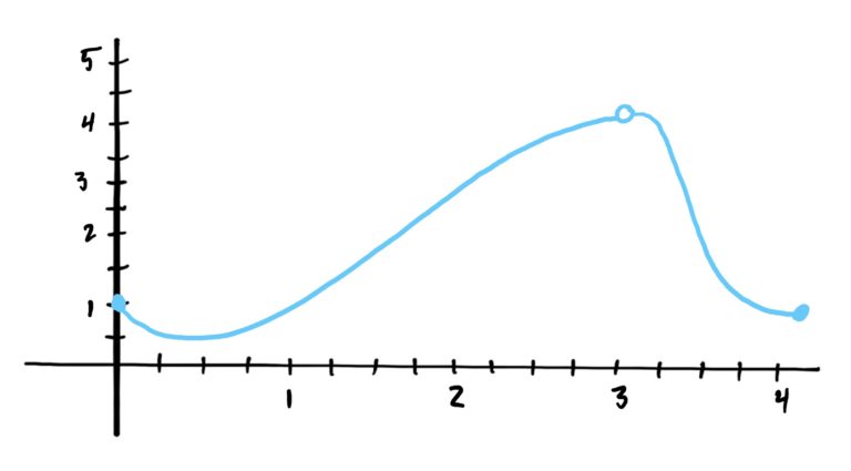
Notice that there is a “hole” in the graph at \(x=3\). Remember that holes in a graph indicate that the function is not defined at that \(x\)-value. However, its really clear what \(y\)-value should be there (i.e. \(y=4\)).

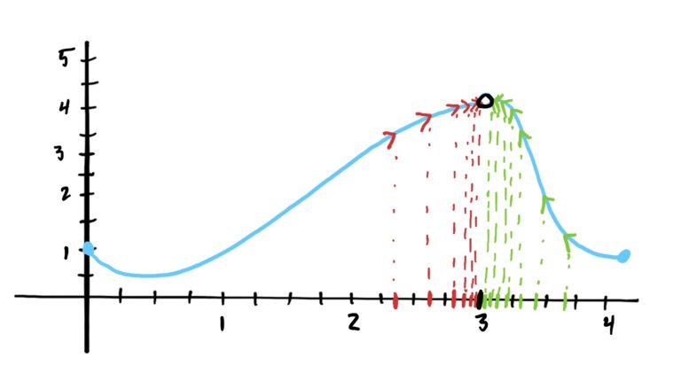
But what about the graph tells us that this is the case? Essentially, to determine the \(y\)-value of the point that should be in the hole, we see where the graph is “headed” on both the right and the left sides of the hole. More explicitly, we are seeing what happens to the \(y\)-values of the function as our \(x\)-values approach the “problem point” \(x=3\). This is indicated by the arrows you see on the graph below.

Our minds basically did all of this “determining where the graph is headed” automatically for us. In the lessons that follow, we make this idea a little more precise. However, the idea remains that simple: “what happens to a function’s \(y\)-values as we get closer and closer to some specific \(x\)-value (or point)?” Keeping this simple idea in mind will help with understanding as we cover limits in more depth.

Limits: A Study of Extremes

Limits can be thought of as a “study of extreme values.” When finding or computing limits, what we are really doing is determining what happens to a function as input \(x\)-values get infinitely small, infinitely large, or infinitely close to a specific value (much like what we saw in the above example with \(x=3\)).

Take a look at the graph below, which represents the population of bacteria on a Petri dish over time.

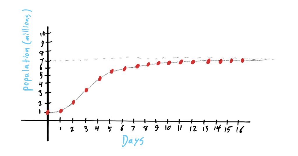
Notice that as time increases (i.e. the \(x\)-value inputs get bigger) the population of bacteria increases, and will always continue to increase (albeit by very little when enough time has passed). However, the population does not increase without bound; that is, the population doesn’t just slowly grow to be “infinity.” It looks like there is a maximum to the number of bacteria that can survive in the Petri dish. In Biology and Ecology, this maximum number is often called a population’s carrying capacity. Looking at this graph, no matter how much time has passed, the population will never reach the carrying capacity, BUT it will get “infinitely close to it” as an “”infinite amount of time” passes. When looking at a graph like this, we can only reasonably surmise that the population will not exceed the \(y\)-value of the dashed line.

Overall, the rules and laws of limits that we will study allow us to concretely determine what happens to functions as inputs get really large, really small, or really close to specific values.