Future Value of Income Streams

Regular Accumulation Over Time

Recall from a previous lesson that we can use the formula

$$P(t)=P_0e^{rt}$$

to determine the value of an asset over time \(t\) that starts at amount \(P_0\), and compounds (continuously) at rate \(r\). We also mentioned in that same lesson that this formula serves as a good approximation and an upper bound for less frequent compounding (such as daily compounding).

Dividend Re-Investing

There are investment vehicles out there that will occasionally pay you back a certain percentage of your initial investment on a regular basis. This may take the form of a stock dividend, a bond coupon, a crypto staking reward, or some other form. While your original investment compounds at a certain rate over time, you can take these payouts and reinvest them along with your original investment, compounding your returns even more! Let’s take a look at an example where we want to determine how much money we have if we reinvest these payouts.

Continuous Payouts? Yes, that can happen… almost.

There are investments out there that pay out “rewards” or dividends on a more frequent basis. In the cryptocurrency/digital asset world, weekly, daily, or even more rapid payouts are commonplace.

Let’s suppose we found an account/investment that compounds continuously at an annual rate of 4% and we invest $2000 in the account. Suppose also that this account pays out a daily reward of $0.05 that you immediately reinvest upon receipt. How much do we have after two years of this process?

The setup is the same as the example above. However, instead of multiplying each term by $0.05/day for the compounding of each payout, we will write instead \(\frac{18.25}{365}\) (which equals (0.05)), where the \(18.25\) is the represents the total payout for one year. The reason we’re doing this will be (hopefully) clear later.

$$Value(t)=2000e^{0.04\cdot (2)}+\frac{18.25}{365}e^{0.04\cdot(2-\frac{1}{365})}+\frac{18.25}{365}e^{0.04\cdot(2-\frac{2}{365})}+…+\frac{18.25}{365}e^{0.04\cdot (2-\frac{730}{365})}$$

This is a lot of adding that would take a good bit of time to plug into a calculator or even write/code into a spreadsheet. What might be beneficial is, instead of adding up 731 different amounts, we just assumed that the account paid out its rewards continuously (i.e. infinitely often). So this gives us the following limit, where we are driving the number of payouts that are infinitely close together to infinity.

$$\lim_{n\rightarrow\infty} 2000e^{0.04\cdot (2)}+\frac{18.25}{n}e^{0.04\cdot(2-\frac{1}{n})}+\frac{18.25}{n}e^{0.04\cdot(2-2\frac{1}{n})}+\frac{18.25}{n}e^{0.04\cdot(2-3\frac{1}{n})}…+\frac{18.25}{n}e^{0.04\cdot (2-\frac{2n}{n})}$$

Cleaning things up a little bit by breaking up the yearly total payout \(18.25\) and the number of times \(n\) we divide that up per year, and letting \(\Delta t =\frac{1}{n}\) (representing how often we get a payout each year) gives us

$$\begin{align}\lim_{n\rightarrow\infty} 2000e^{0.04\cdot (2)}+18.25e^{0.04\cdot(2-1\cdot \Delta t)}\cdot \Delta t+…+18.25e^{0.04\cdot (2-2n\cdot \Delta t)}\cdot \Delta t \end{align}$$

When we take limits of sums of stuff that is getting infinitely close together, we end up with an integral! This makes sense because are continuously accumulating these rewards, and integrals “sum up” continuous accumulation.

$$\begin{align}\lim_{n\rightarrow\infty} 2000e^{0.04\cdot (2)}+18.25e^{0.04\cdot(2-1\cdot \Delta t)}\cdot \Delta t+…+18.25e^{0.04\cdot (2-2n\cdot \Delta t)}\cdot \Delta t&=\int^2_0 18.25 e^{0.04\cdot(2-t)}\ dt \end{align}$$

Since you cannot receive rewards more than continuously, the above integral gives us an upper bound for how much money we will have in our account after two years. Since there is likely to be little difference in what we’d get if we received daily payouts versus continuous payouts, computing the above integral also gives us a good estimate for the value of our account after 2 years. Below is the computation of the integral part.

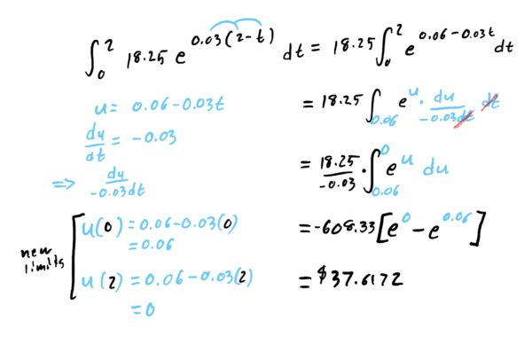
Thus, the total value of the account after two years is given by

$$Value(2)=2000e^{0.04\cdot (2)}+37.6172=2204.19$$

In general, we can use the following integral formula to determine the value of a continuously compounding investment that has continuous (or “fast enough” payouts). Again, this is useful for finding upper bounds for accounts with less frequent compoundings.