Graphing Piecewise-Defined Functions Copy
Mini Lecture Video
Key Takeaways
Recall that a piecewise defined function (or just “piecewise function,” colloquially) is a function that is built from using different function rules depending on the given input value. The output of the rule that corresponds to a particular input value is the value of the entire piecewise function on that input.
For example, let
$$
f(x)=\begin{cases}
x^2 & x\leq 0 \\
2x+1 & 0<x\leq 10 \\
x^3 & 10< x
\end{cases}
$$
If you wanted to find the output of the function above on input \(x=2\), we notice that of the three conditions listed on the right-hand-side of the function’s definition, the second condition of \(0<x\leq 10\) is the one that applies if \(x=2\). So, to produce a \(y\)-value for the function \(f\) at \(x=2\), we plug \(x=2\) into the second function.
Noting that all the piecewise function’s \(y\)-values come from plugging inputs into each piece of the function, we can graph piecewise functions essentially by plotting points, or alternatively by graphing each piece separately, but only keeping the part of the graph that falls above the \(x\)-values given by the condition beside that piece. The mini video lecture illustrates how to do this; as do each of the examples below.
Try the Following!
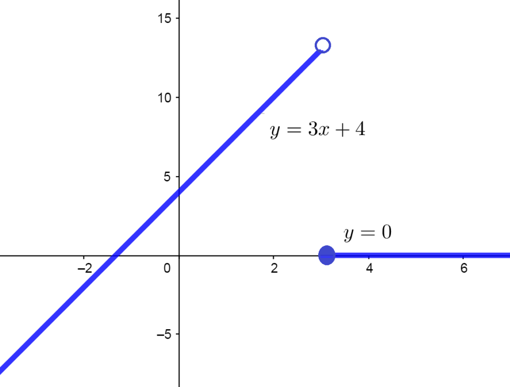
$$
f(x)=\begin{cases}
3x+4 & x<3 \\
0 & 3\leq x
\end{cases}
$$
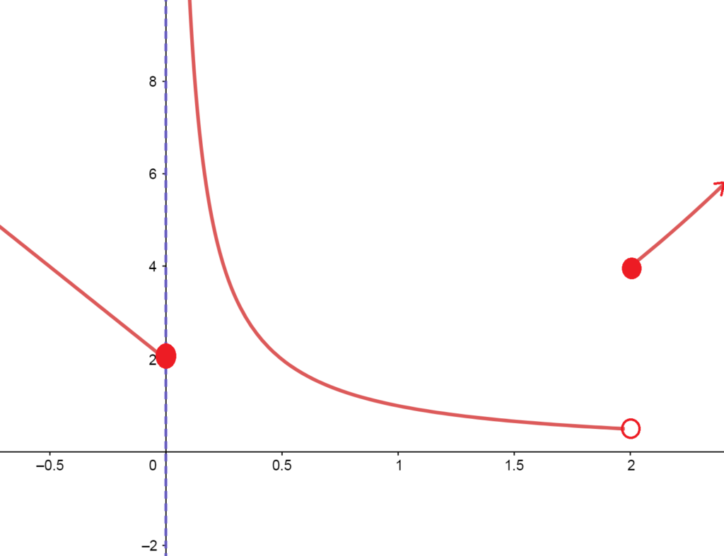
$$
g(x)=\begin{cases}
-4x+2 & x\leq 0 \\
\frac{1}{x} & 0<x<2 \\
x^2 & x\geq 2
\end{cases}
$$
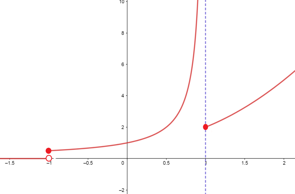
$$
f(x)=\begin{cases}
0 & x\leq -1 \\
\frac{1}{1-x} & -1< x< 1 \\
x^2+1 & 1\leq x
\end{cases}
$$